266 : Periodic Navier–Stokes

(source code)

This example solves the incompressible Navier–Stokes equations with periodic boundary conditions between inlet and outlet, and no-slip boundary conditions on the other walls. The equations seek a velocity $\mathbf{u}$ and a pressure $p$ such that

\[\begin{aligned} - \mu \Delta \mathbf{u} + (\mathbf{u} \cdot \nabla) \mathbf{u} + \nabla p & = \mathbf{f}\\ \mathrm{div}(\mathbf{u}) & = 0 \end{aligned}\]

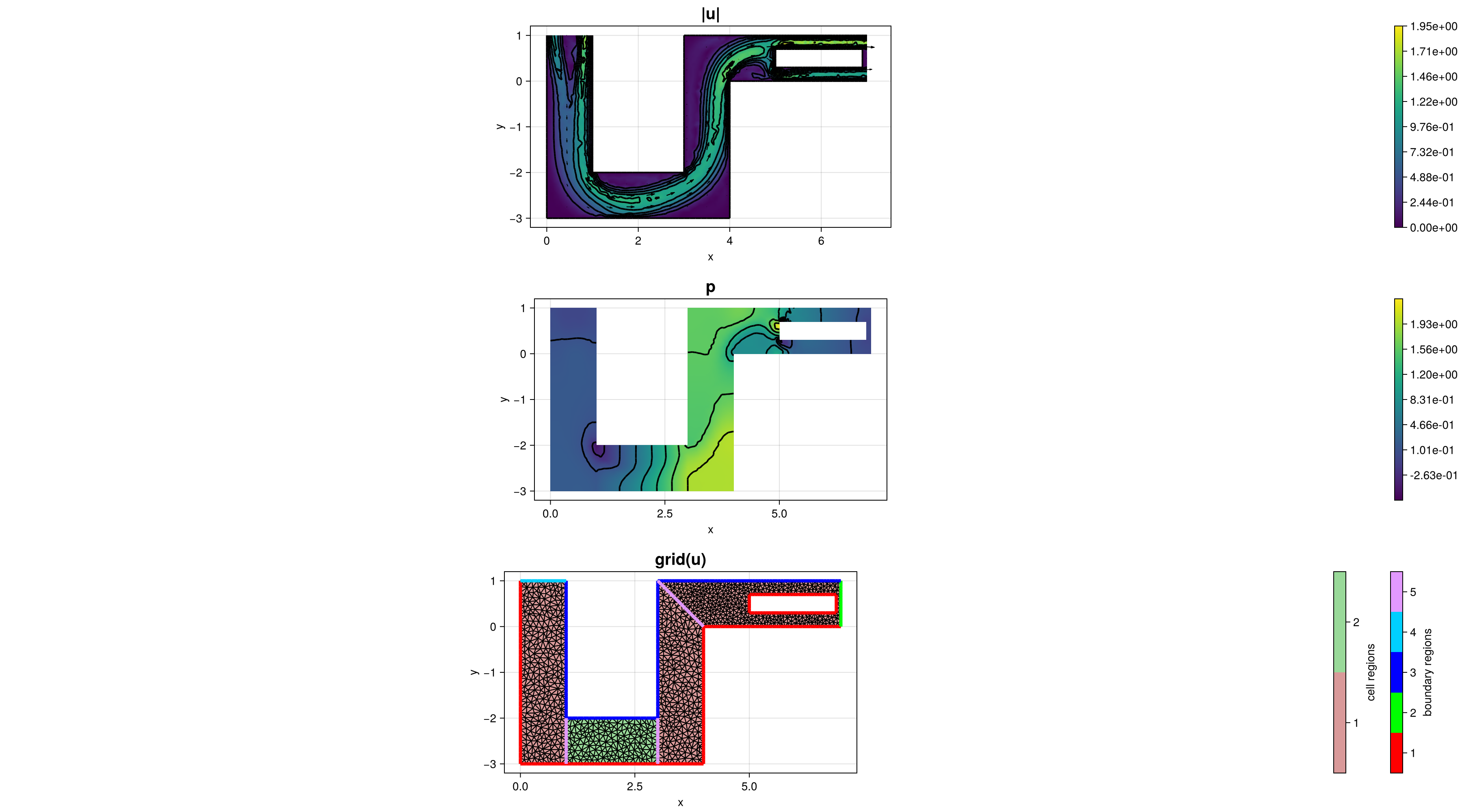
The solution is computed via Taylor–Hood elements. For the default parameters the result looks like this:

module Example266_PeriodicNavierStokes

using ExtendableFEM
using ExtendableFEMBase
using ExtendableGrids
using SimplexGridFactory
using Triangulate
using UnicodePlots; import Term

# kernel for the nonlinear Navier--Stokes operator
# residuals: [convection, Stokes x, Stokes y, divergence]
function kernel_nonlinear!(result, u_ops, qpinfo)
    u, ∇u, p = view(u_ops, 1:2), view(u_ops, 3:6), view(u_ops, 7)
    μ = qpinfo.params[1]
    result[1] = dot(u, view(∇u, 1:2))
    result[2] = dot(u, view(∇u, 3:4))
    result[3] = μ * ∇u[1] - p[1]
    result[4] = μ * ∇u[2]
    result[5] = μ * ∇u[3]
    result[6] = μ * ∇u[4] - p[1]
    result[7] = -(∇u[1] + ∇u[4])
    return nothing
end

# source term: horizontal body force
function f_body!(result, qpinfo)
    result[1] = 1.0
    result[2] = 0.0
    return nothing
end

# everything is wrapped in a main function
function main(;
        maxvol = 1.0e-2,
        Plotter = UnicodePlots,
        μ = 3.0e-3,
        periodic = true,
        nrefs = 0,
        kwargs...
    )

    # load mesh and refine
    xgrid = uniform_refine(
        simplexgrid(
            Triangulate;
            points = [0 1; 0 -3; 1 -3; 3 -3; 4 -3; 4 0; 7 0; 7 1; 3 1; 3 -2; 1 -2; 1 1; 5 0.3; 6.9 0.3; 6.9 0.7; 5 0.7]',
            bfaces = [1 2; 2 3; 3 4; 4 5; 5 6; 6 7; 7 8; 8 9; 9 10; 10 11; 11 12; 12 1; 3 11; 4 10; 13 14; 14 15; 15 16; 16 13; 6 9]',
            bfaceregions = [1; 1; 1; 1; 1; 1; 2; 3; 3; 3; 3; 4; 5; 5; 1; 1; 1; 1; 5],
            regionpoints = [0.5 0.5; 2.0 -2.5; 3.5 -2.5; 6.99 0.5; 6.5 0.5]',
            regionnumbers = [1, 2, 1, 1, 0],
            regionvolumes = [1, 1, 1, 0.5, 0] * maxvol
        ),
        nrefs
    )

    # define unknowns
    u = Unknown("u"; name = "velocity", dim = 2)
    p = Unknown("p"; name = "pressure", dim = 1)

    # problem description
    PD = ProblemDescription("Periodic Navier--Stokes problem")
    assign_unknown!(PD, u)
    assign_unknown!(PD, p)

    # nonlinear Navier--Stokes operator (includes convection + Stokes + continuity)
    assign_operator!(
        PD, NonlinearOperator(
            kernel_nonlinear!, [id(u), grad(u), id(p)];
            params = [μ], kwargs...
        )
    )

    # body force in the x-direction
    assign_operator!(PD, LinearOperator(f_body!, [id(u)]; regions = [2], kwargs...))

    function target2source!(y, x)
        y[1] = 7.0
        y[2] = x[1]
        return nothing
    end

    function post_mutation!(result, input, qpinfo)
        result[1] = input[2]
        result[2] = -input[1]
        return result
    end

    # periodic coupling
    periodic && assign_restriction!(
        PD, CoupledDofsRestriction(
            u, 2, 4;
            target2source!,
            post_mutation!
        )
    )

    # no-slip on top and bottom walls
    assign_operator!(PD, HomogeneousBoundaryData(u; regions = [1, 3], kwargs...))

    # fix one pressure dof
    assign_operator!(PD, FixDofs(p; dofs = [1], vals = [0]))

    # generate FESpaces and solution vector
    FES = [FESpace{H1P2{2, 2}}(xgrid), FESpace{H1P1{1}}(xgrid)]

    sol = ExtendableFEM.solve(PD, FES, damping = 0.5, maxiterations = 5) # start with damping
    sol = ExtendableFEM.solve(PD, FES, init = sol, maxiterations = 100)

    # plot
    plt = plot([id(u), id(p), grid(u)], sol; Plotter = Plotter, ncols = 1, rasterpoints = 1000, width = 1800, height = 1000)

    test_points = [
        ([7.0, 0.15], [0.15, 1.0]),
        ([7.0, 0.5], [0.5, 1.0]),
        ([7.0, 0.85], [0.85, 1.0]),
    ]

    PE = PointEvaluator([id(u)], sol)

    err = 0.0
    for points in test_points
        y = zeros(2)
        evaluate!(y, PE, points[1])
        z = zeros(2)
        post_mutation!(z, y, nothing)
        evaluate!(y, PE, points[2])
        err += norm(z - y)^2
    end

    return sol, plt, err
end


end # module

This page was generated using Literate.jl.