220 : Heat Equation (implicit Euler, mixed geometries)
This example computes the solution $u$ of the two-dimensional heat equation
\[\begin{aligned} u_t - \mu \Delta u & = f \quad \text{in } \Omega \times (0, T] \\ u \lvert_{\partial \Omega} & = 0 \\ u(\cdot, 0) & = u_0 \end{aligned}\]
on the unit square $\Omega$ on a grid with mixed geometries (grid_unitsquare_mixedgeometries builds the unit square from a mix of triangle and parallelogram cells).
The time integration uses the implicit (backward) Euler scheme
\[\frac{u^{n+1} - u^n}{\tau} - \mu \, \Delta u^{n+1} = f(\cdot, t^{n+1}), \qquad \tau = T / n,\]
which gives the linear system
\[(M + \tau \, \mu \, K) \, u^{n+1} = M \, u^n + \tau \, b^{n+1}\]
with mass matrix $M = (\Phi_j, \Phi_i)$, stiffness matrix $K = (\nabla \Phi_j, \nabla \Phi_i)$ and right-hand side $b^{n+1} = (f(\cdot, t^{n+1}), \Phi_i)$. The implicit Euler scheme is unconditionally stable.
The spatial discretization uses the mixed geometry Lagrange element $H1Q1$ ($P1$ space on triangles, $Q1$ space on parallelograms). The local-to-global assembly of $M$, $K$ and $b$ is written low-level, i.e. as explicit assembly loops with one typed (allocation-free) inner loop per unique cell geometry.
The computed solution for the default parameters with initial condition $u_0(x) = \sin(\pi x_1) \sin(\pi x_2)$ (exact solution $u(x,t) = \mathrm{e}^{-2 \pi^2 t} \sin(\pi x_1) \sin(\pi x_2)$) looks like this:
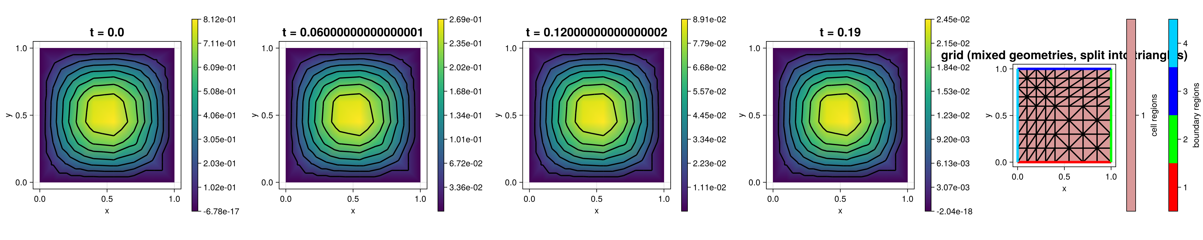
Since the plotter used in the docs build (CairoMakie) can only plot triangle cells, the solution is interpolated onto a P1 space on a triangle-only grid obtained from the mixed grid via split_grid_into before plotting.
module Example220_LowLevelHeatEquation

using ExtendableFEMBase
using ExtendableGrids
using ExtendableSparse
using GridVisualize
using UnicodePlots, Term
using Test #

# initial condition (vanishes on the boundary)
function u0!(result, qpinfo)
    x = qpinfo.x
    return result[1] = sin(π * x[1]) * sin(π * x[2])
end

# exact solution of the default problem: u(x, t) = exp(-2π² μ t) sin(π x₁) sin(π x₂)
function uexact!(result, qpinfo)
    x = qpinfo.x
    t = qpinfo.time
    return result[1] = exp(-2.0 * π * π * t) * sin(π * x[1]) * sin(π * x[2])
end

function main(;
        nref = 2,
        T = 0.2,
        nsteps = 20,
        mu = 1.0,
        rhs = (x, t) -> 0.0,
        Plotter = UnicodePlots,
    )
    # Finite element type: mixed geometry Lagrange element (P1 on triangles, Q1 on parallelograms)
    FEType = H1Q1{1}

    # grid with mixed geometries (triangle and parallelogram cells)
    xgrid = uniform_refine(grid_unitsquare_mixedgeometries(), nref)

    # FESpace
    fe_space = FESpace{FEType}(xgrid)

    # solve
    history = solve_heat_lowlevel(fe_space, u0!, rhs, mu, T, nsteps)

    # separate grid for plotting: the plotter used in the docs build (CairoMakie)
    # can only plot triangle cells, so split the mixed grid into triangles and
    # interpolate the solution onto a P1 space on the plot grid
    xgridplot = split_grid_into(xgrid, Triangle2D)
    fe_space_plot = FESpace{H1P1{1}}(xgridplot)

    # plot four time levels and the grid
    plotsteps = [1]
    append!(plotsteps, [round(Int, nsteps * j / 3) for j in 1:3])
    plt = GridVisualizer(; Plotter = Plotter, layout = (1, length(plotsteps) + 1), clear = true, resolution = (400 * (length(plotsteps) + 1), 400))
    for (j, n) in enumerate(plotsteps)
        u_plot = FEVector(fe_space_plot; name = "u(t = $(T * (n - 1) / nsteps)) on plot grid")
        lazy_interpolate!(u_plot[1], history[n + 1]; use_cellparents = true)
        scalarplot!(plt[1, j], u_plot[1], title = "t = $(T * (n - 1) / nsteps)")
    end
    gridplot!(plt[1, length(plotsteps) + 1], xgridplot; markersize = 0, title = "grid (mixed geometries, split into triangles)")
    reveal(plt)

    return history, plt
end


function solve_heat_lowlevel(fe_space, u0!, rhs, mu, T, nsteps)
    tau = T / nsteps
    ndofs = fe_space.ndofs

    # assemble mass matrix M and system matrix A = M + τ μ K once
    println("Assembling...")
    M = FEMatrix(fe_space, fe_space)
    fill_mass!(M.entries, fe_space)
    A = FEMatrix(fe_space, fe_space)
    fill_system!(A.entries, fe_space, mu, tau)

    # fix homogeneous Dirichlet boundary dofs
    bdofs = boundarydofs(fe_space)
    for dof in bdofs
        A.entries[dof, dof] = 1.0e60
    end
    ExtendableSparse.flush!(A.entries)

    # interpolate initial condition
    u = FEVector(fe_space; name = "u(t = 0)")
    interpolate!(u[1], u0!)
    un = copy(u.entries)
    history = [u]

    b = zeros(Float64, ndofs)
    for n in 1:nsteps
        t = n * tau

        # right-hand side: M u^n + τ (rhs(·, t), ·)
        rhsvec = M.entries.cscmatrix * un
        fill!(b, 0)
        fill_rhs!(b, fe_space, rhs, t, tau)
        rhsvec .+= b
        for dof in bdofs
            rhsvec[dof] = 0
        end

        # solve linear system
        un = A.entries \ rhsvec

        push!(history, FEVector(fe_space; entries = un, name = "u(t = $(t))"))
    end

    return history
end


# ------------------------------------------------------------------
# low-level assembly on grids with mixed geometries:
# one typed (barrier) function per unique cell geometry, so that
# the inner assembly loop is allocation-free
# ------------------------------------------------------------------

# mass matrix: M[i,j] = ∫Ω Φ_i Φ_j
function fill_mass!(M::ExtendableSparseMatrix, fe_space::FESpace{Tv, Ti}) where {Tv, Ti}
    xgrid = fe_space.xgrid
    FEType = eltype(fe_space)
    cellvolumes = xgrid[CellVolumes]
    celldofs = fe_space[CellDofs]
    xCellGeometries = xgrid[CellGeometries]

    loop_allocations = 0
    for EG in xgrid[UniqueCellGeometries]
        # quadrature formula (exact for the product of two basis functions)
        qf = QuadratureRule{Float64, EG}(2 * max(1, get_polynomialorder(FEType, EG) - 1))
        weights::Vector{Float64} = qf.w
        nweights::Int = length(weights)

        # FE basis evaluator
        FEBasis_id = FEEvaluator(fe_space, Identity, qf)
        idvals = FEBasis_id.cvals

        function barrier(EG::Type{<:AbstractElementGeometry})
            # barrier function to avoid allocations by type dispatch
            ndofs4cell::Int = get_ndofs(ON_CELLS, FEType, EG)
            Mloc = zeros(Float64, ndofs4cell, ndofs4cell)
            ncells::Int = num_cells(xgrid)
            dof_j::Int, dof_k::Int = 0, 0

            return loop_allocations += @allocated for cell::Ti in 1:ncells
                # skip cells of other element geometries (mixed geometry grids)
                if xCellGeometries[cell] !== EG
                    continue
                end

                # update FE basis evaluator
                FEBasis_id.citem[] = cell
                update_basis!(FEBasis_id)

                # assemble local mass matrix
                for j in 1:ndofs4cell, k in j:ndofs4cell
                    temp = 0
                    for qp in 1:nweights
                        temp += weights[qp] * idvals[1, j, qp] * idvals[1, k, qp]
                    end
                    Mloc[j, k] = temp
                end
                Mloc .*= cellvolumes[cell]

                # add local matrix to global matrix
                for j in 1:ndofs4cell
                    dof_j = celldofs[j, cell]
                    for k in j:ndofs4cell
                        dof_k = celldofs[k, cell]
                        rawupdateindex!(M, +, Mloc[j, k], dof_j, dof_k)
                        if k > j
                            rawupdateindex!(M, +, Mloc[j, k], dof_k, dof_j)
                        end
                    end
                end
                fill!(Mloc, 0)
            end
        end
        barrier(EG)
    end
    ExtendableSparse.flush!(M)
    return loop_allocations
end

# system matrix for implicit Euler: A = M + τ μ K
function fill_system!(A::ExtendableSparseMatrix, fe_space::FESpace{Tv, Ti}, mu = 1.0, tau = 1.0) where {Tv, Ti}
    xgrid = fe_space.xgrid
    FEType = eltype(fe_space)
    cellvolumes = xgrid[CellVolumes]
    celldofs = fe_space[CellDofs]
    xCellGeometries = xgrid[CellGeometries]

    loop_allocations = 0
    for EG in xgrid[UniqueCellGeometries]
        # quadrature formula (exact for the products of basis functions and gradients)
        qf = QuadratureRule{Float64, EG}(2 * max(1, get_polynomialorder(FEType, EG) - 1))
        weights::Vector{Float64} = qf.w
        nweights::Int = length(weights)

        # FE basis evaluators
        FEBasis_∇ = FEEvaluator(fe_space, Gradient, qf)
        ∇vals = FEBasis_∇.cvals
        FEBasis_id = FEEvaluator(fe_space, Identity, qf)
        idvals = FEBasis_id.cvals

        function barrier(EG::Type{<:AbstractElementGeometry})
            # barrier function to avoid allocations by type dispatch
            ndofs4cell::Int = get_ndofs(ON_CELLS, FEType, EG)
            Aloc = zeros(Float64, ndofs4cell, ndofs4cell)
            ncells::Int = num_cells(xgrid)
            dof_j::Int, dof_k::Int = 0, 0

            return loop_allocations += @allocated for cell::Ti in 1:ncells
                # skip cells of other element geometries (mixed geometry grids)
                if xCellGeometries[cell] !== EG
                    continue
                end

                # update FE basis evaluators
                FEBasis_∇.citem[] = cell
                update_basis!(FEBasis_∇)
                FEBasis_id.citem[] = cell
                update_basis!(FEBasis_id)

                # assemble local system matrix M + τ μ K
                for j in 1:ndofs4cell, k in j:ndofs4cell
                    tempM = 0
                    tempK = 0
                    for qp in 1:nweights
                        tempM += weights[qp] * idvals[1, j, qp] * idvals[1, k, qp]
                        tempK += weights[qp] * dot(view(∇vals, :, j, qp), view(∇vals, :, k, qp))
                    end
                    Aloc[j, k] = tempM + tau * mu * tempK
                end
                Aloc .*= cellvolumes[cell]

                # add local matrix to global matrix
                for j in 1:ndofs4cell
                    dof_j = celldofs[j, cell]
                    for k in j:ndofs4cell
                        dof_k = celldofs[k, cell]
                        rawupdateindex!(A, +, Aloc[j, k], dof_j, dof_k)
                        if k > j
                            rawupdateindex!(A, +, Aloc[j, k], dof_k, dof_j)
                        end
                    end
                end
                fill!(Aloc, 0)
            end
        end
        barrier(EG)
    end
    ExtendableSparse.flush!(A)
    return loop_allocations
end

# right-hand side: b[i] = τ (f(·, t), Φ_i)
function fill_rhs!(b::Vector, fe_space::FESpace{Tv, Ti}, rhs, t = 0.0, tau = 1.0) where {Tv, Ti}
    xgrid = fe_space.xgrid
    FEType = eltype(fe_space)
    cellvolumes = xgrid[CellVolumes]
    celldofs = fe_space[CellDofs]
    xCellGeometries = xgrid[CellGeometries]

    loop_allocations = 0
    for EG in xgrid[UniqueCellGeometries]
        # quadrature formula
        qf = QuadratureRule{Float64, EG}(2 * max(1, get_polynomialorder(FEType, EG) - 1))
        weights::Vector{Float64} = qf.w
        xref::Vector{Vector{Float64}} = qf.xref
        nweights::Int = length(weights)

        # FE basis evaluator and local2global transformation
        L2G = L2GTransformer(EG, xgrid, ON_CELLS)
        FEBasis_id = FEEvaluator(fe_space, Identity, qf)
        idvals = FEBasis_id.cvals

        function barrier(EG::Type{<:AbstractElementGeometry}, L2G::L2GTransformer)
            # barrier function to avoid allocations by type dispatch
            ndofs4cell::Int = get_ndofs(ON_CELLS, FEType, EG)
            ncells::Int = num_cells(xgrid)
            dof_j::Int = 0
            x::Vector{Float64} = zeros(Float64, 2)

            return loop_allocations += @allocated for cell::Ti in 1:ncells
                # skip cells of other element geometries (mixed geometry grids)
                if xCellGeometries[cell] !== EG
                    continue
                end

                # update FE basis evaluator and transformation
                FEBasis_id.citem[] = cell
                update_basis!(FEBasis_id)
                update_trafo!(L2G, cell)

                # assemble local right-hand side
                for j in 1:ndofs4cell
                    temp = 0
                    for qp in 1:nweights
                        # get global x for quadrature point
                        eval_trafo!(x, L2G, xref[qp])
                        temp += weights[qp] * idvals[1, j, qp] * rhs(x, t)
                    end
                    # write into global vector
                    dof_j = celldofs[j, cell]
                    b[dof_j] += temp * cellvolumes[cell] * tau
                end
            end
        end
        barrier(EG, L2G)
    end
    return loop_allocations
end


function generateplots(dir = pwd(); Plotter = nothing, kwargs...)
    ~, plt = main(; Plotter = Plotter, kwargs...)
    scene = GridVisualize.reveal(plt)
    return GridVisualize.save(joinpath(dir, "example220.png"), scene; Plotter = Plotter)
end

# tests: allocation-free assembly of the low-level loops on the mixed
# geometry grid, monotonic energy decay of the implicit Euler scheme,
# and the error against the exact solution
function runtests(;
        nref = 1,
        T = 0.2,
        nsteps = 20,
        mu = 1.0,
    )
    FEType = H1Q1{1}
    xgrid = uniform_refine(grid_unitsquare_mixedgeometries(), nref)
    fe_space = FESpace{FEType}(xgrid)
    tau = T / nsteps

    # the low-level assembly loops should be allocation-free
    # after the first pass, which fills the sparse pattern
    M = FEMatrix(fe_space, fe_space)
    @info "allocations in 1st mass assembly: $(fill_mass!(M.entries, fe_space))"
    @test fill_mass!(M.entries, fe_space) == 0

    A = FEMatrix(fe_space, fe_space)
    @info "allocations in 1st system assembly: $(fill_system!(A.entries, fe_space, mu, tau))"
    @test fill_system!(A.entries, fe_space, mu, tau) == 0

    b = zeros(Float64, fe_space.ndofs)
    @info "allocations in 1st rhs assembly: $(fill_rhs!(b, fe_space, (x, t) -> 0.0, 0.0, tau))"
    @test fill_rhs!(b, fe_space, (x, t) -> 0.0, 0.0, tau) == 0

    # solve over the time interval
    history = solve_heat_lowlevel(fe_space, u0!, (x, t) -> 0.0, mu, T, nsteps)

    # discrete energy should decay monotonically (rhs = 0, homogeneous Dirichlet)
    Mmat = M.entries.cscmatrix
    En = [0.5 * history[n].entries' * (Mmat * history[n].entries) for n in 1:length(history)]
    @test all(diff(En) .<= 1.0e-12)
    #@test En[end] < 0.01 * En[1]

    # error at time T against the FEM interpolation of the exact solution
    uex = FEVector(fe_space)
    interpolate!(uex[1], uexact!; time = T)
    e = history[end].entries .- uex.entries
    err2 = e' * (Mmat * e)
    @info "error in mass norm at t = T: $(sqrt(err2))"
    @test isapprox(sqrt(err2), 5.320626237289539e-4; rtol = 1.0e-10)
    return nothing
end #module
This page was generated using Literate.jl.